Gradient descent

src: i.ytimg.com

Gradient descent is a first-order iterative optimization algorithm for finding the minimum of a function. To find a local minimum of a function using gradient descent, one takes steps proportional to the negative of the gradient (or approximate gradient) of the function at the current point. If instead one takes steps proportional to the positive of the gradient, one approaches a local maximum of that function; the procedure is then known as gradient ascent.

Gradient descent is also known as steepest descent. However, gradient descent should not be confused with the method of steepest descent for approximating integrals.

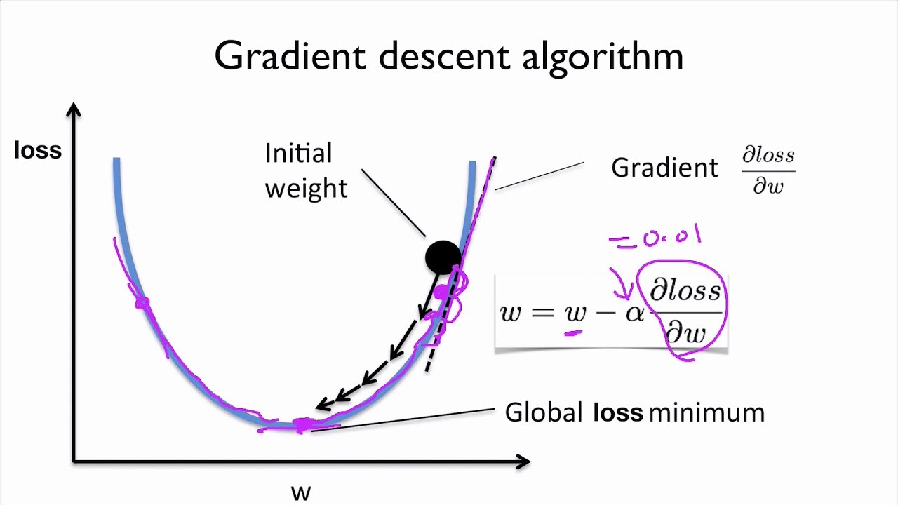
Video Gradient descent

Description

Gradient descent is based on the observation that if the multi-variable function ${\displaystyle F(\mathbf {x} )}$ is defined and differentiable in a neighborhood of a point ${\displaystyle \mathbf {a} }$, then ${\displaystyle F(\mathbf {x} )}$ decreases fastest if one goes from ${\displaystyle \mathbf {a} }$ in the direction of the negative gradient of ${\displaystyle F}$ at ${\displaystyle \mathbf {a} }$, ${\displaystyle -\nabla F(\mathbf {a} )}$. It follows that, if

${\displaystyle \mathbf {a} _{n+1}=\mathbf {a} _{n}-\gamma \nabla F(\mathbf {a} _{n})}$

for ${\displaystyle \gamma }$ small enough, then ${\displaystyle F(\mathbf {a_{n}} )\geq F(\mathbf {a_{n+1}} )}$. In other words, the term ${\displaystyle \gamma \nabla F(\mathbf {a} )}$ is subtracted from ${\displaystyle \mathbf {a} }$ because we want to move against the gradient, toward the minimum. With this observation in mind, one starts with a guess ${\displaystyle \mathbf {x} _{0}}$ for a local minimum of ${\displaystyle F}$, and considers the sequence ${\displaystyle \mathbf {x} _{0},\mathbf {x} _{1},\mathbf {x} _{2},\dots }$ such that

${\displaystyle \mathbf {x} _{n+1}=\mathbf {x} _{n}-\gamma _{n}\nabla F(\mathbf {x} _{n}),\ n\geq 0.}$

We have

${\displaystyle F(\mathbf {x} _{0})\geq F(\mathbf {x} _{1})\geq F(\mathbf {x} _{2})\geq \cdots ,}$

so hopefully the sequence ${\displaystyle (\mathbf {x} _{n})}$ converges to the desired local minimum. Note that the value of the step size ${\displaystyle \gamma }$ is allowed to change at every iteration. With certain assumptions on the function ${\displaystyle F}$ (for example, ${\displaystyle F}$ convex and ${\displaystyle \nabla F}$ Lipschitz) and particular choices of ${\displaystyle \gamma }$ (e.g., chosen either via a line search that satisfies the Wolfe conditions or the Barzilai-Borwein method shown as following),

${\displaystyle \gamma _{n}={\frac {(\mathbf {x} _{n}-\mathbf {x} _{n-1})^{T}[\nabla F(\mathbf {x} _{n})-\nabla F(\mathbf {x} _{n-1})]}{||\nabla F(\mathbf {x} _{n})-\nabla F(\mathbf {x} _{n-1})||^{2}}}}$

convergence to a local minimum can be guaranteed. When the function ${\displaystyle F}$ is convex, all local minima are also global minima, so in this case gradient descent can converge to the global solution.

This process is illustrated in the adjacent picture. Here ${\displaystyle F}$ is assumed to be defined on the plane, and that its graph has a bowl shape. The blue curves are the contour lines, that is, the regions on which the value of ${\displaystyle F}$ is constant. A red arrow originating at a point shows the direction of the negative gradient at that point. Note that the (negative) gradient at a point is orthogonal to the contour line going through that point. We see that gradient descent leads us to the bottom of the bowl, that is, to the point where the value of the function ${\displaystyle F}$ is minimal.

Examples

Gradient descent has problems with pathological functions such as the Rosenbrock function shown here.

${\displaystyle f(x_{1},x_{2})=(1-x_{1})^{2}+100(x_{2}-{x_{1}}^{2})^{2}.\quad }$

The Rosenbrock function has a narrow curved valley which contains the minimum. The bottom of the valley is very flat. Because of the curved flat valley the optimization is zig-zagging slowly with small stepsizes towards the minimum.

The "Zig-Zagging" nature of the method is also evident below, where the gradient descent method is applied to ${\displaystyle F(x,y)=\sin \left({\frac {1}{2}}x^{2}-{\frac {1}{4}}y^{2}+3\right)\cos(2x+1-e^{y})}$.

Limitations

For some of the above examples, gradient descent is relatively slow close to the minimum: technically, its asymptotic rate of convergence is inferior to many other methods. For poorly conditioned convex problems, gradient descent increasingly 'zigzags' as the gradients point nearly orthogonally to the shortest direction to a minimum point. For more details, see the comments below.

For non-differentiable functions, gradient methods are ill-defined. For locally Lipschitz problems and especially for convex minimization problems, bundle methods of descent are well-defined. Non-descent methods, like subgradient projection methods, may also be used. These methods are typically slower than gradient descent. Another alternative for non-differentiable functions is to "smooth" the function, or bound the function by a smooth function. In this approach, the smooth problem is solved in the hope that the answer is close to the answer for the non-smooth problem (occasionally, this can be made rigorous).

Maps Gradient descent

Solution of a linear system

Gradient descent can be used to solve a system of linear equations, reformulated as a quadratic minimization problem, e.g., using linear least squares. The solution of

${\displaystyle A\mathbf {x} -\mathbf {b} =0}$

in the sense of linear least squares is defined as minimizing the function

${\displaystyle F(\mathbf {x} )=\|A\mathbf {x} -\mathbf {b} \|^{2}.}$

In traditional linear least squares for real ${\displaystyle A}$ and ${\displaystyle \mathbf {b} }$ the Euclidean norm is used, in which case

${\displaystyle \nabla F(\mathbf {x} )=2A^{T}(A\mathbf {x} -\mathbf {b} ).}$

In this case, the line search minimization, finding the locally optimal step size ${\displaystyle \gamma }$ on every iteration, can be performed analytically, and explicit formulas for the locally optimal ${\displaystyle \gamma }$ are known.

For solving linear equations, this algorithm is rarely used, with the conjugate gradient method being one of the most popular alternatives. The speed of convergence of gradient descent depends on the ratio of the maximum to minimum eigenvalues of ${\displaystyle A^{T}A}$, while the speed of convergence of conjugate gradients has a more complex dependence on the eigenvalues, and can benefit from preconditioning. Gradient descent also benefits from preconditioning, but this is not done as commonly.

src: steemitimages.com

Solution of a non-linear system

Gradient descent can also be used to solve a system of nonlinear equations. Below is an example that shows how to use the gradient descent to solve for three unknown variables, x₁, x₂, and x₃. This example shows one iteration of the gradient descent.

Consider the nonlinear system of equations

${\displaystyle {\begin{cases}3x_{1}-\cos(x_{2}x_{3})-{\tfrac {3}{2}}=0\\4x_{1}^{2}-625x_{2}^{2}+2x_{2}-1=0\\\exp(-x_{1}x_{2})+20x_{3}+{\tfrac {10\pi -3}{3}}=0.\end{cases}}}$

Let us introduce the associated function

${\displaystyle G(\mathbf {x} )={\begin{bmatrix}3x_{1}-\cos(x_{2}x_{3})-{\tfrac {3}{2}}\\4x_{1}^{2}-625x_{2}^{2}+2x_{2}-1\\\exp(-x_{1}x_{2})+20x_{3}+{\tfrac {10\pi -3}{3}}\\\end{bmatrix}}}$,

where

${\displaystyle \mathbf {x} ={\begin{bmatrix}x_{1}\\x_{2}\\x_{3}\\\end{bmatrix}}}$.

One might now define the objective function

${\displaystyle F(\mathbf {x} )={\tfrac {1}{2}}G^{\mathrm {T} }(\mathbf {x} )G(\mathbf {x} )={\tfrac {1}{2}}\left(\left(3x_{1}-\cos(x_{2}x_{3})-{\tfrac {3}{2}}\right)^{2}+\left(4x_{1}^{2}-625x_{2}^{2}+2x_{2}-1\right)^{2}+\left(\exp(-x_{1}x_{2})+20x_{3}+{\tfrac {1}{3}}(10\pi -3)\right)^{2}\right)}$,

which we will attempt to minimize. As an initial guess, let us use

${\displaystyle \mathbf {x} ^{(0)}={\begin{bmatrix}0\\0\\0\\\end{bmatrix}}}$.

We know that

${\displaystyle \mathbf {x} ^{(1)}=\mathbf {x} ^{(0)}-\gamma _{0}\nabla F(\mathbf {x} ^{(0)})}$,

where

${\displaystyle \nabla F(\mathbf {x} ^{(0)})=J_{G}(\mathbf {x} ^{(0)})^{\mathrm {T} }G(\mathbf {x} ^{(0)})}$.

The Jacobian matrix ${\displaystyle J_{G}}$ is given by

${\displaystyle J_{G}(\mathbf {x} )={\begin{bmatrix}3&\sin(x_{2}x_{3})x_{3}&\sin(x_{2}x_{3})x_{2}\\8x_{1}&-1250x_{2}+2&0\\-x_{2}\exp {(-x_{1}x_{2})}&-x_{1}\exp(-x_{1}x_{2})&20\\\end{bmatrix}}}$.

Evaluating ${\displaystyle J_{G}}$ and ${\displaystyle G}$ at ${\displaystyle \mathbf {x} ^{(0)}}$ yields

${\displaystyle J_{G}\left(\mathbf {x} ^{(0)}\right)={\begin{bmatrix}3&0&0\\0&2&0\\0&0&20\end{bmatrix}},\qquad G(\mathbf {x} ^{(0)})={\begin{bmatrix}-2.5\\-1\\10.472\end{bmatrix}}}$.

Thus,

${\displaystyle \mathbf {x} ^{(1)}=0-\gamma _{0}{\begin{bmatrix}-7.5\\-2\\209.44\end{bmatrix}}}$

and

${\displaystyle F\left(\mathbf {x} ^{(0)}\right)=0.5\left((-2.5)^{2}+(-1)^{2}+(10.472)^{2}\right)=58.456}$.

Now, a suitable ${\displaystyle \gamma _{0}}$ must be found such that ${\displaystyle F(\mathbf {x} ^{(1)})\leq F(\mathbf {x} ^{(0)})}$. This can be done with any of a variety of line search algorithms. One might also simply guess ${\displaystyle \gamma _{0}=0.001}$, which gives

${\displaystyle \mathbf {x} ^{(1)}={\begin{bmatrix}0.0075\\0.002\\-0.20944\\\end{bmatrix}}}$.

Evaluating the objective function at this value, yields

${\displaystyle F\left(\mathbf {x} ^{(1)}\right)=0.5\left((-2.48)^{2}+(-1.00)^{2}+(6.28)^{2}\right)=23.306}$.

The decrease from ${\displaystyle F(\mathbf {x} ^{(0)})=58.456}$ to the next step's value of ${\displaystyle F(\mathbf {x} ^{(1)})=23.306}$ is a sizable decrease in the objective function. Further steps would reduce its value further, until an approximate solution to the system was found.

src: i.ytimg.com

Gradient descent works in spaces of any number of dimensions, even in infinite-dimensional ones. In the latter case the search space is typically a function space, and one calculates the Fréchet derivative of the functional to be minimized to determine the descent direction.

The gradient descent can take many iterations to compute a local minimum with a required accuracy, if the curvature in different directions is very different for the given function. For such functions, preconditioning, which changes the geometry of the space to shape the function level sets like concentric circles, cures the slow convergence. Constructing and applying preconditioning can be computationally expensive, however.

The gradient descent can be combined with a line search, finding the locally optimal step size ${\displaystyle \gamma }$ on every iteration. Performing the line search can be time-consuming. Conversely, using a fixed small ${\displaystyle \gamma }$ can yield poor convergence.

Methods based on Newton's method and inversion of the Hessian using conjugate gradient techniques can be better alternatives. Generally, such methods converge in fewer iterations, but the cost of each iteration is higher. An example is the BFGS method which consists in calculating on every step a matrix by which the gradient vector is multiplied to go into a "better" direction, combined with a more sophisticated line search algorithm, to find the "best" value of ${\displaystyle \gamma .}$ For extremely large problems, where the computer memory issues dominate, a limited-memory method such as L-BFGS should be used instead of BFGS or the steepest descent.

Gradient descent can be viewed as Euler's method for solving ordinary differential equations ${\displaystyle x'(t)=-\nabla f(x(t))}$ of a gradient flow.

src: www.mathworks.com

Computational examples

Python

The gradient descent algorithm is applied to find a local minimum of the function f(x)=x⁴-3x³+2, with derivative f'(x)=4x³-9x². Here is an implementation in the Python programming language.

Scala

Here is an implementation in Scala programming language

Julia

Here is the same algorithm implemented in the Julia programming language.

C

Here is the same algorithm implemented in the C programming language.

The above piece of code has to be modified with regard to step size according to the system at hand and convergence can be made faster by using an adaptive step size. In the above case the step size is not adaptive. It stays at 0.01 in all the directions which can sometimes cause the method to fail by diverging from the minimum.

Javascript (ES6)

Here is an example of gradient descent against randomised values, squareMeter and price, written in Javascript

MATLAB

The following MATLAB code demonstrates a concrete solution for solving the non-linear system of equations presented in the previous section:

${\displaystyle {\begin{cases}3x_{1}-\cos(x_{2}x_{3})-{\tfrac {3}{2}}=0\\4x_{1}^{2}-625x_{2}^{2}+2x_{2}-1=0\\\exp(-x_{1}x_{2})+20x_{3}+{\tfrac {10\pi -3}{3}}=0\end{cases}}}$

R

The following R code is an example of implementing gradient descent algorithm to find the minimum of the function f(x)=x⁴-3x³+2 in previous section. Note that we are looking for f(x)'s minimum by solving its derivative being equal to zero.

${\displaystyle \nabla f(x)=4x^{3}-9x^{2}=0}$

And the x can be updated with gradient descent method every iteration in the form of

${\displaystyle x^{(k+1)}=x^{(k)}-\alpha \nabla f(x^{(k)})}$

where k = 1, 2, ..., maximum iteration, and ? is the step size.

src: i.ytimg.com

Extensions

Gradient descent can be extended to handle constraints by including a projection onto the set of constraints. This method is only feasible when the projection is efficiently computable on a computer. Under suitable assumptions, this method converges. This method is a specific case of the forward-backward algorithm for monotone inclusions (which includes convex programming and variational inequalities).

Fast gradient methods

Another extension of gradient descent is due to Yurii Nesterov from 1983, and has been subsequently generalized. He provides a simple modification of the algorithm that enables faster convergence for convex problems. For unconstrained smooth problems the method is called the Fast Gradient Method (FGM) or the Accelerated Gradient Method (AGM). Specifically, if the differentiable function ${\displaystyle F}$ is convex and ${\displaystyle \nabla F}$ is Lipschitz, and it is not assumed that ${\displaystyle F}$ is strongly convex, then the error in the objective value generated at each step ${\displaystyle k}$ by the gradient descent method will be bounded by ${\displaystyle {\mathcal {O}}(1/k)}$. Using the Nesterov acceleration technique, the error decreases at ${\displaystyle {\mathcal {O}}(1/k^{2})}$. It is known that the rate ${\displaystyle {\mathcal {O}}(1/k^{2})}$ for the decrease of the cost function is optimal for first-order optimization methods. Nevertheless, there is the opportunity to improve the algorithm by reducing the constant factor. The optimized gradient method (OGM) reduces that constant by a factor of two and is an optimal first-order method for large-scale problems.

For constrained or non-smooth problems, Nesterov's FGM is called the fast proximal gradient method (FPGM), an acceleration of the proximal gradient method.

The momentum method

Yet another extension, that reduces the risk of getting stuck in a local minimum, as well as speeds up the convergence considerably in cases where the process would otherwise zig-zag heavily, is the momentum method, which uses a momentum term in analogy to "the mass of Newtonian particles that move through a viscous medium in a conservative force field". This method is often used as an extension to the backpropagation algorithms used to train artificial neural networks.

src: d3c33hcgiwev3.cloudfront.net

An analogy for understanding gradient descent

The basic intuition behind gradient descent can be illustrated by a hypothetical scenario. A person is stuck in the mountains and is trying to get down (i.e. trying to find the minima). There is heavy fog such that visibility is extremely low. Therefore, the path down the mountain is not visible, so he must use local information to find the minima. He can use the method of gradient descent, which involves looking at the steepness of the hill at his current position, then proceeding in the direction with the steepest descent (i.e. downhill). If he was trying to find the top of the mountain (i.e. the maxima), then he would proceed in the direction steepest ascent (i.e. uphill). Using this method, he would eventually find his way down the mountain. However, assume also that the steepness of the hill is not immediately obvious with simple observation, but rather it requires a sophisticated instrument to measure, which the person happens to have at the moment. It takes quite some time to measure the steepness of the hill with the instrument, thus he should minimize his use of the instrument if he wanted to get down the mountain before sunset. The difficulty then is choosing the frequency at which he should measure the steepness of the hill so not to go off track.

In this analogy, the person represents the algorithm, and the path taken down the mountain represents the sequence of parameter settings that the algorithm will explore. The steepness of the hill represents the slope of the error surface at that point. The instrument used to measure steepness is differentiation (the slope of the error surface can be calculated by taking the derivative of the squared error function at that point). The direction he chooses to travel in aligns with the gradient of the error surface at that point. The amount of time he travels before taking another measurement is the learning rate of the algorithm. See the limitation section for a discussion of the limitations of this type of "hill climbing" algorithm.

src: i.ytimg.com

See also

• Conjugate gradient method
• Stochastic gradient descent
• Rprop
• Delta rule
• Wolfe conditions
• Preconditioning
• BFGS method
• Nelder-Mead method
• Gauss-Newton algorithm
• Hill climbing

src: s-media-cache-ak0.pinimg.com

References

src: i.ytimg.com

Sources

• Avriel, Mordecai (2003). Nonlinear Programming: Analysis and Methods. Courier Corporation. ISBN 978-0-486-43227-4. 
• Snyman, Jan (3 March 2005). Practical Mathematical Optimization: An Introduction to Basic Optimization Theory and Classical and New Gradient-Based Algorithms. Springer Science & Business Media. ISBN 978-0-387-24348-1. 
• Homod, Raad Z.; Sahari, Khairul Salleh Mohamed; Almurib, Haider A. F.; Nagi, Farrukh Hafiz (2012-06-01). "Gradient auto-tuned Takagi-Sugeno Fuzzy Forward control of a HVAC system using predicted mean vote index". Energy and Buildings. 49 (6): 254-267. doi:10.1016/j.enbuild.2012.02.013. 
• Cauchy, Augustin (1847). Méthode générale pour la résolution des systèmes d'équations simultanées. pp. 536-538. 

src: i1.wp.com

External links

• Using gradient descent in C++, Boost, Ublas for linear regression
• Series of Khan Academy videos discusses gradient ascent
• Online book teaching gradient descent in deep neural network context

Source of the article : Wikipedia